Why Infrared ISP Is Harder Than a Sensor Swap
Replacing a visible-light sensor with an uncooled thermal detector changes more than the pixel format. An infrared ISP must separate scene information from pixel non-uniformity and the camera’s changing thermal state, then deliver useful data for viewing, measurement or machine perception.
INFRARED IMAGE PROCESSING / SYSTEM DESIGN
The difficult part is the coupling.
NUC, drift compensation, denoising and contrast enhancement cannot be tuned independently. An error left by one stage can become a convincing false detail at the next. Good architecture starts by defining the signal, the calibration state and the output each application needs.
1. The input includes the scene and the camera
This article focuses on uncooled LWIR microbolometers, such as VOx arrays used in thermal camera modules. It does not describe every infrared detector: SWIR photon sensors and cooled MWIR systems have different operating requirements.
A microbolometer absorbs infrared energy, heats a thermally isolated pixel and reads the resulting resistance change. The received signal includes object emission, reflected surroundings and atmospheric effects. The camera’s optics and housing can contribute thermal radiation too.
yᵢ(t) ≈ gᵢ(s) × Lᵢ(t) + oᵢ(s) + nᵢ(t)
Lᵢ: received in-band scene radiance
gᵢ, oᵢ: pixel-dependent response and offset
s: camera state, including focal-plane temperature and operating mode
nᵢ: noise
This is a simplified engineering model, not a universal calibration equation. It explains why a stationary target can produce changing counts while the camera warms up. Scene radiance and internal response cannot always be uniquely separated from an image alone; reference measurements, calibration and temperature telemetry supply additional information.
A study of long-term shutterless microbolometer stability found that lens-housing temperature, alongside focal-plane temperature, mattered to the tested camera’s radiometric model. The practical lesson is to characterize the assembled thermal system.
2. Compare engineering tasks, not stereotypes
Visible-light ISPs also solve difficult low-light, HDR, noise, calibration and machine-vision problems. They do not receive perfectly stable pixels, and they do more than make images attractive. Basler’s flat-field correction documentation, for example, covers dark-signal and photo-response non-uniformity in visible cameras.
The useful comparison is how an uncooled thermal detector changes the engineering priorities.
| Design question | Visible-light ISP | Uncooled LWIR ISP |
|---|---|---|
| Signal origin | Often reflected illumination; depends on application | In-band thermal emission, reflections and path contributions |
| Pixel correction | Black level, shading, bad pixels, DSNU / PRNU as required | Pixel NUC and thermally dependent residual correction are central |
| Camera state | Exposure, gain, temperature, optics and illumination matter | FPA and assembly temperatures can alter response and self-emission |
| Display processing | Color or monochrome processing, tone mapping, NR and detail | AGC / DRC, NR, detail and optional false color |
| Measurement output | Application-specific calibration and image data | Radiometric temperature requires its own calibration and model |
| Runtime correction | Depends on camera and application | May use shutter references, temperature models or scene-based methods |
There is no universal non-uniformity percentage, ADC width or drift coefficient that defines either category. A drift value in LSB/°C is incomplete without the gain, digital scale, integration setting and operating range. Compare specified conditions before comparing numbers.
3. NUC and FFC make the pixel responses comparable
When a uniform source produces a spatial pattern, the image contains structure from the instrument. Non-uniformity correction, or NUC, reduces pixel-to-pixel response differences. A simple correction is xᵢ = aᵢ × yᵢ + bᵢ, with coefficients established for the relevant operating state.
Two-point calibration uses two uniform reference levels to estimate a gain and offset mapping. Multi-point or temperature-indexed calibration can cover a wider response range, with added acquisition, storage and validation work. A bad-pixel map identifies unusable samples; replacement can improve continuity but does not recover an independent measurement at the defective pixel.
In a shutter-based flat-field correction, or FFC, a reference surface temporarily fills the detector’s view so the camera can refresh its correction. A single reference observation is commonly used for an offset update; it does not independently determine both gain and offset. The flag is not automatically a traceable absolute-temperature standard.
AT Sensors’ microbolometer guide describes factory pixel calibration, runtime offset updates and shutterless compensation as distinct parts of the correction chain.
Design runtime correction as a managed process: track the coefficient set, relevant temperatures and correction events. FFC may interrupt or freeze the scene stream, so downstream recording and analysis need an explicit policy for those frames. A mechanical shutter is one implementation, not a requirement of every thermal camera.
4. Display compression can amplify the wrong information
High-bit-depth samples and an 8-bit display solve different problems. A 14-bit code space has 16,384 possible values; an 8-bit grayscale display has 256. Mapping between them does not make each gray level a fixed temperature increment, and it cannot recover a saturated detector signal.
Automatic gain control and dynamic range compression choose which differences remain visible. Histogram methods, clipped or plateau histograms, and local contrast methods allocate the display range differently. Base/detail approaches compress broad intensity variation while preserving smaller structures. A published infrared DRC method uses this separation to address contrast and noise together.
The coupling matters: residual pixel patterns can enter the detail layer along with real edges. Aggressive local gain then makes instrument structure easier to see. Check flat-field residuals before interpreting stronger texture as improved scene detail.
Use the right radiation model. Stefan–Boltzmann’s σT⁴ law describes total blackbody emission integrated over all wavelengths, with temperature in kelvin. An LWIR camera samples a limited spectral band. Its counts depend on band response, optics, emissivity and operating state; they do not simply follow σT⁴. FLIR’s thermography reference explains the distinction between spectral and total radiation.
Thermal scenes can be demanding, but there is no general rule that their dynamic range exceeds every visible HDR scene. Specify the temperatures, apparent contrast and saturation limits your application must handle.
5. Temperature compensation belongs in the architecture
Warm-up, changing ambient conditions and electronics self-heating can alter the detector response. A calibration valid in one thermal state may leave residual error in another. Research on temperature-dependent microbolometer non-uniformity describes models that use camera temperature to compensate those changing patterns.
Two different design choices are often confused:
- TEC-stabilized versus TEC-less: whether a thermoelectric device actively regulates the detector assembly’s temperature.
- Shutter-based versus shutterless: whether a blocking reference flag is used during runtime correction.
Removing a TEC does not automatically remove the shutter. Removing the shutter does not remove the need for calibration. A shutterless design may combine temperature-dependent models, reference pixels and scene-based correction; its suitability depends on the implementation and scene conditions. Electronic exposure control alone does not present a uniform optical reference to the array.
For the system designer, useful state includes available FPA or housing temperatures, their rate of change, operating range, coefficient version and time since a relevant reference update. These are candidate engineering signals, not a mandatory universal interface. Provide the telemetry, storage access and scheduling needed by the chosen correction strategy.
Good steady-state imagery is only one acceptance condition. Test after power-on and during thermal transitions, including the actual enclosure, heat sources and airflow. A smooth display may conceal a drift that still matters to measurement or long-running analysis.
6. Denoising must preserve the task-relevant signal
NETD describes thermal sensitivity under defined test conditions. 30–50 mK corresponds to 0.03–0.05°C of temperature difference; it does not mean ±0.03–0.05°C absolute measurement accuracy. FLIR lists thermal sensitivity and accuracy as different camera specifications.
A 1°C target-to-background difference is not automatically close to a 30 mK noise floor. In practice, apparent contrast can shrink when a target fills only part of a pixel, optics spread the signal, the atmosphere attenuates it, or the viewing geometry changes. Evaluate the received image and target sampling rather than inferring detection performance from two headline temperatures.
Spatial denoising trades random variation against small-feature preservation. Temporal denoising can improve a stationary image while leaving trails on moving objects. Motion-adaptive weights and edge-aware filters are useful options, but their behavior must be tested for the intended task.
Measure uniformity, temporal noise, edge response and motion artifacts separately. Do not ask a downstream smoother to hide every upstream calibration problem. For a radiometric output, validate that filtering preserves the measurement behavior required by the application; the display’s preferred smoothing is not automatically the measurement path’s preferred smoothing.
7. Keep display, analysis and temperature data distinct
A common failure sequence is easy to follow: residual NUC error becomes local texture, local contrast increases that texture, and sharpening emphasizes its boundaries. A second failure begins with a thermal transition: counts shift, a downstream threshold remains fixed, and a previously stable decision changes.
These examples suggest a practical debugging order. Inspect data before and after correction, filtering and display mapping. Log the camera state alongside those frames. Compare a uniform reference with a real scene so the source of structure is easier to isolate.
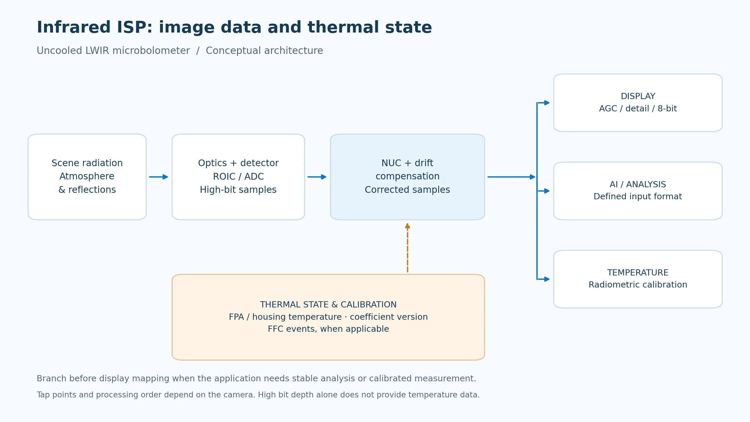
The output contract should identify three possible consumers:
- Display: tone mapping, detail enhancement, overlays and optional palettes produce a useful presentation.
- AI or host analysis: choose a defined sample format and preprocessing path, then use a consistent pipeline for training and deployment. An AI model may use 8-bit images or higher-bit-depth samples; neither is universally required.
- Temperature measurement: use a radiometrically calibrated camera and its documented conversion and object parameters. Emissivity and reflected apparent temperature affect the result, as FLIR’s measurement documentation explains.
A 16-bit container is not a temperature unit. Nor does “RAW” identify a universal pipeline tap. It may refer to detector-side, corrected, pre-AGC or another vendor-defined output. Define meaningful bit depth, scaling, packing, invalid samples and calibration metadata before designing the consumer.
Residual-error estimates or local noise maps can help later stages limit enhancement. Treat that as a design option to evaluate, rather than assuming every ISP exposes a calibrated per-pixel confidence map.
8. Algorithms, memory and scheduling must be designed together
Three levels of work meet here. The algorithm defines the correction and filtering model. The hardware pipeline decides precision, buffering, arithmetic and parallelism. The SoC integration schedules sensor input, coefficient access, CPU control, memory and optional inference.
A small calculation makes the resource question concrete. Assume 640 × 512 pixels at 50 frames/s, 16-bit frame storage and one 16-bit gain plus one 16-bit offset per pixel. These are illustrative design choices, not the specifications of an internal CAMCUDA ISP.
| Resource | Calculation | Result |
|---|---|---|
| One stored frame | 640 × 512 × 2 bytes | 655,360 bytes · 0.625 MiB |
| Gain and offset maps | 640 × 512 × 2 maps × 2 bytes | 1,310,720 bytes · 1.25 MiB |
| One sequential frame stream | 655,360 × 50 | 32.768 MB/s |
| One frame read plus write per cycle | 2 × 655,360 × 50 | 65.536 MB/s |
| Coefficient reads, if fetched every frame | 1,310,720 × 50 | 65.536 MB/s |
| One history read plus write per cycle | 2 × 655,360 × 50 | 65.536 MB/s |
If all three read/write-and-coefficient operations above reach external memory independently, their sum is 196.608 MB/s, before other consumers and overhead. This is a deliberately simple traffic model. Streaming stages, on-chip storage, caching and buffer reuse can change the external traffic substantially. MB uses 1,000,000 bytes; MiB uses 1,048,576 bytes.
Frame histories add memory and can add latency; coefficient precision affects residual error; range-dependent LUTs need versioning and safe updates. NPU traffic competes with image buffers only when the chosen system shares those resources. Build the budget from the actual dataflow instead of declaring every infrared SoC a sub-1 W design.
Validate the coupled system
Run a uniform-source test, a warm-up or ambient-transition test, a small moving-target sequence and a scene containing both low-contrast detail and a bright thermal object. For each, record the output mode, calibration state, frame timestamps, dropped or reference frames, latency and relevant image metrics. Add blackbody accuracy testing when the delivered camera is radiometric.
The goal is a reproducible operating envelope: a defined image or measurement output that stays useful while scene content and camera state change.
Choose a CAMCUDA module around the required data
The same detector resolution can support different integration goals. These three modules illustrate the distinction between host-side grayscale processing, shutterless imaging and a specified radiometric camera.
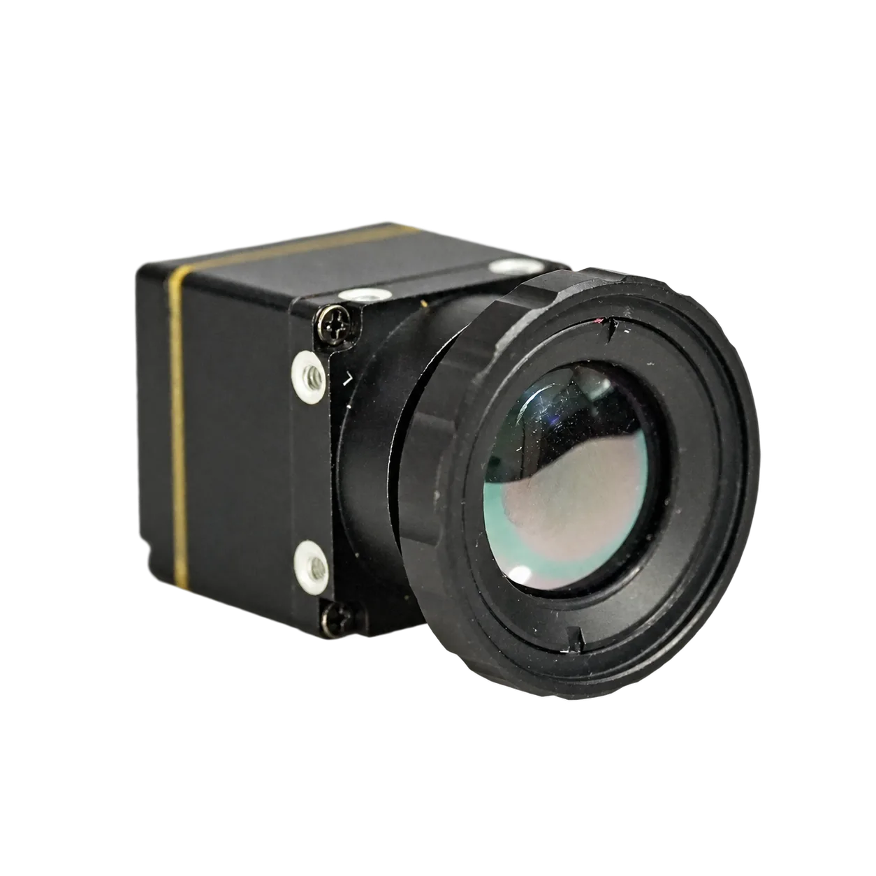
FlexMini 640: keep the analysis buffer separate
The 640 × 512, 12 μm FlexMini 640 provides a documented USB UVC Y16 workflow: Y14 grayscale in a 16-bit container. RAW, pre-AGC and post-AGC source selection depends on firmware capabilities. Preserve the original capture for processing; the grayscale stream is not calibrated temperature output.
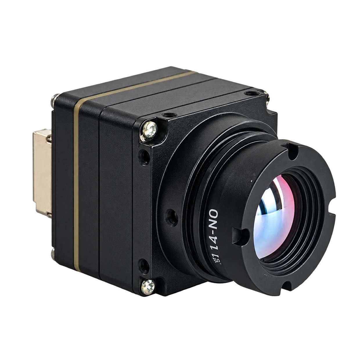
HI640: evaluate shutterless imaging
HI640 combines a 640 × 512, 12 μm VOx detector with shutterless NUC and a listed 50 Hz detector rate. Its specification lists USB, MIPI-CSI and CVBS paths. Evaluate warm-up, environmental changes and actual host output with the selected configuration; shutterless operation does not establish radiometric capability.
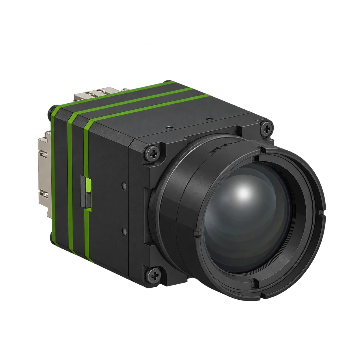
ThermoCore 640: specify a radiometric data path
ThermoCore 640 is offered as a 640 × 512, 12 μm radiometric module with 25 Hz imaging and a −20°C to +150°C measurement range. Its product documentation lists 14/16-bit USB RAW output and SDK AGC levels 0–5, with level 0 disabling AGC. Request the matched SDK, sample file and conversion details for your host.
| Integration question | FlexMini 640 14-bit RAW · Y16 |
HI640 Shutterless imaging |
ThermoCore 640 Radiometric USB RAW |
|---|---|---|---|
| Detector | 640 × 512 · 12 μm | 640 × 512 · 12 μm | 640 × 512 · 12 μm |
| Published rate reference | 50 Hz; capture mode is configuration-dependent | 50 Hz detector rate; host mode to confirm | 25 Hz radiometric imaging |
| Relevant output feature | Y14 grayscale in USB UVC Y16 | Shutterless NUC; USB / MIPI-CSI / CVBS references | 14/16-bit USB RAW and SDK AGC control |
| Temperature data | Documented RAW path is non-radiometric | Calibrated measurement is not specified | Radiometric configuration · −20°C to +150°C |
Product references reviewed 25 October 2026. Confirm the supplied firmware, interface and capture format with the selected assembly. Detector frame rates and bit-depth labels alone do not establish sustained host capture or a temperature conversion formula.
Continue with the FlexMini 640 RAW capture guide, the shutterless module comparison or the thermal FOV calculation explainer.
Frequently asked questions
Why is an infrared ISP more than a visible sensor replacement?
An uncooled microbolometer couples scene radiation with pixel response differences and camera thermal state. Its correction, drift compensation and output requirements must be designed together rather than inherited unchanged from a visible-light pipeline.
Does every thermal camera need a mechanical FFC shutter?
No. Shutter-based systems use a reference flag, while shutterless systems use other compensation methods. Both still need an appropriate calibration and runtime correction strategy.
Are shutterless and TEC-less the same thing?
No. Shutterless describes the absence of a blocking correction flag. TEC-less describes the absence of thermoelectric temperature stabilization. They are separate design choices.
Does a 30 mK NETD mean ±0.03°C measurement accuracy?
No. 30 mK equals a 0.03°C temperature difference, but NETD is a sensitivity metric under stated conditions. Absolute temperature accuracy also depends on radiometric calibration, environment and measurement settings.
Does 14-bit or 16-bit RAW automatically contain temperatures?
No. Bit depth and storage format do not define radiometric units. The camera must provide calibrated measurement data or a documented conversion with the required calibration and object parameters.
Must a thermal AI model use high-bit-depth RAW?
No. A model can use display images or higher-bit-depth samples. Choose an input path that supports the task and keep its format and preprocessing consistent between training and deployment.
Sources and engineering notes
- AT Sensors: Microbolometer basics — detector operation and correction concepts.
- Basler: Flat-field correction — DSNU and PRNU correction in visible cameras.
- Wolf, Pezoa and Figueroa: Modeling and Compensating Temperature-Dependent Non-Uniformity Noise in IR Microbolometer Cameras, Sensors, 2016.
- Long-Term Radiometric Stability of Uncooled and Shutterless Microbolometer-Based Infrared Cameras, 2024.
- Dynamic range compression and detail enhancement algorithm for infrared image, Applied Optics, 2014 — base/detail processing example.
- FLIR: Thermography reference documentation — radiation theory and measurement concepts.
- FLIR: Thermal camera specifications — sensitivity and accuracy.
- FLIR: Measuring temperatures — radiometric functionality and measurement parameters.
- CAMCUDA FlexMini 64014-bit RAW · Y16, HI640Shutterless imaging and ThermoCore 640Radiometric USB RAW product specifications.
The block diagram and memory calculation are explanatory engineering examples. They do not disclose or benchmark a product’s internal ISP, calibration coefficients or memory implementation.
Define the output before choosing the module.
Tell us whether you need a viewing stream, grayscale samples for processing, or calibrated temperature data. Include your host, interface, frame rate, scene conditions and quantity so the module and documentation can be matched to the project.