FLIR Boson Integration Guide: Pinouts, Sync Setup & OEM Module Alternatives
FLIR Boson Integration Guide: Pinouts, Sync Setup & OEM Module Alternatives
Integrating an uncooled Long-Wave Infrared (LWIR) core into custom drone gimbals, robotic rovers, or edge AI payloads isn’t like dropping in a standard visible webcam. While the FLIR Boson has spent years as the recognizable benchmark for 12 µm uncooled Vanadium Oxide (VOx) microbolometers, taking a bare thermal core from an evaluation bench kit into a rugged, high-volume production build comes with serious hardware headaches. Between routing high-density mezzanine connectors, wrestling with kernel-level Video4Linux2 (V4L2) drivers in embedded Linux and ROS 2, keeping high-frequency power ripple out of sensitive analog bias lines, and dealing with export red tape, engineering teams run into real-world bottlenecks fast.
Look, building a bulletproof thermal vision system takes more than just bolting a module onto a carrier board. You need a solid grasp of high-density pinout routing, external hardware frame synchronization (EXT_SYNC) for multi-sensor timestamping, zero-copy embedded host pipelines, and viable drop-in OEM alternatives. Whether you are building synchronized thermal stereo vision for GPS-denied visual SLAM, putting together low-latency targeting optics, or cutting down SWaP-C (Size, Weight, Power, and Cost) on a stabilized airborne gimbal, this guide gives you a field-tested integration roadmap alongside production-ready hardware alternatives from the Camcuda Thermal Imaging Portfolio.
Table of Contents
- 👉 1. Electrical Interface, High-Density Pinouts & Carrier Board Design
- 👉 2. Digital Video Transport: MIPI CSI-2, USB UVC, and Industrial Standards
- 👉 3. Hardware Synchronization (EXT_SYNC) for Stereo Thermal & Multi-Sensor Fusion
- 👉 4. Embedded Host Integration: Jetson, Raspberry Pi, ROS 2 & Edge AI Acceleration
- 👉 5. OEM Core Showcase: Camcuda MD-64CA 640×512 Thermal Camera Module
- 👉 6. Portable Field Instrument: Camcuda Handheld Infrared Thermal Observation Device
- 👉 7. Architectural Specification Matrix: FLIR Boson vs. Camcuda Solutions
- 👉 8. SWaP-C Optimization, Optical Path Engineering & Johnson Criteria Sizing
- 👉 9. Deep-Dive Technical FAQ & Hardware Troubleshooting
1. Electrical Interface, High-Density Pinouts & Carrier Board Design
Uncooled LWIR cores pack high-speed digital video, low-speed command UART/I2C buses, external trigger lines, and delicate DC bias rails into miniature multi-pin mezzanine interfaces—most commonly 80-pin Hirose DF40 connectors or Samtec high-density arrays. When you’re spinning a custom carrier PCB for an autonomous payload, schematic partitioning and board layout discipline will make or break your signal integrity.
Here’s the deal on high-speed routing: the digital video interface—whether configured for MIPI CSI-2 D-PHY or CMOS parallel—is unforgiving. For MIPI D-PHY lanes, differential clock and data pairs must hit a target impedance of 100 $\Omega$ ($\pm 10\%$). Keep intra-pair skew under 0.15 mm (6 mils) and run them over a continuous, unbroken ground reference plane. If you run USB 2.0 High-Speed lines (D+/D-), maintain a clean 90 $\Omega$ differential profile. Don’t let these traces cross plane splits, and keep them well clear of inductive motor drivers or buck-boost coils.
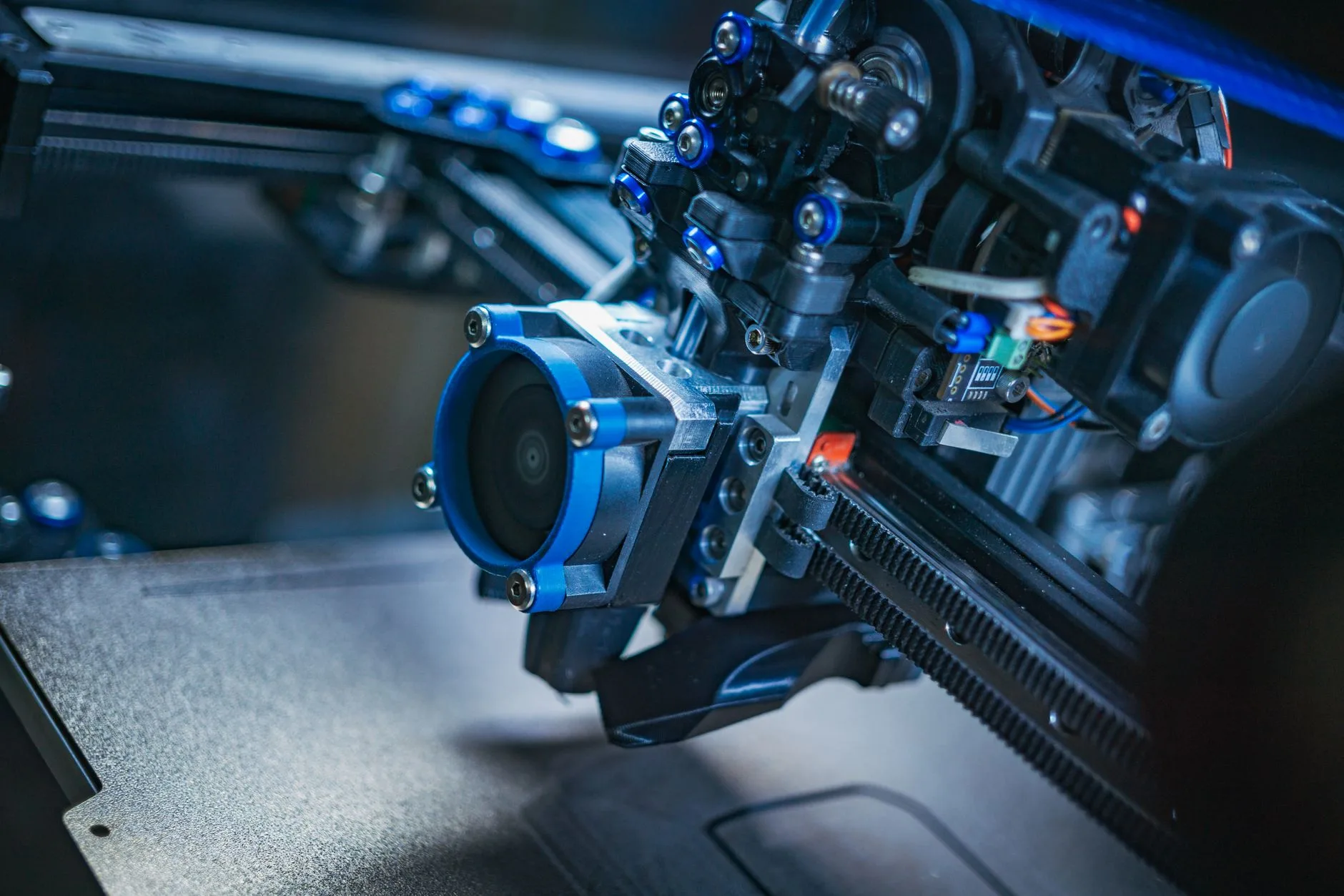
Power delivery network (PDN) design is where many bench prototypes run into trouble. Microbolometer focal plane arrays (FPAs) read minute resistance shifts across tiny micro-machined Vanadium Oxide bridges via on-die Readout Integrated Circuits (ROICs). High-frequency switching noise on your DC input rail ($<100\,\text{kHz}$ to $2\,\text{MHz}$) from cheap switching regulators will bleed right into the analog-to-digital stage. On your thermal monitor, this turns up as ugly horizontal banding, fixed-pattern noise (FPN) drift, and ruined Noise Equivalent Temperature Difference (NETD).
To keep your thermal video clean and free of electrical noise artifacts:
- ⚙️ Keep Input Ripple Ultra-Low: Total voltage ripple on the core input rail must stay below 15 mV peak-to-peak under dynamic processing loads.
- ⚙️ Isolate Core Power Rails: Isolate sensitive camera logic from noisy servo and ESC motor buses by using dedicated Low-Dropout Linear Regulators (LDOs) with high Power Supply Rejection Ratios (PSRR $> 65\,\text{dB}$ at $100\,\text{kHz}$).
- ⚙️ Optimize Decoupling Placement: Drop low-ESR ceramic decoupling capacitors ($0.1\,\mu\text{F}$ and $10\,\mu\text{F}$ X7R/X5R) right next to the mezzanine connector power pins to kill high-frequency ringing before it enters the core.
- ⚙️ Preserve Ground Integrity: Maintain a solid, uninterrupted ground return plane on Layer 2 directly beneath your signal layer to prevent parasitic ground loops and cross-talk.
2. Digital Video Transport: MIPI CSI-2, USB UVC, and Industrial Standards
Choosing your video interface comes down to three operational parameters: system latency, host processor overhead, and the physical cable run between the sensor optical head and your computing unit.
MIPI CSI-2 (Camera Serial Interface): For tight robotics payloads, NVIDIA Jetson modules, and embedded Linux SoCs, MIPI CSI-2 is king. Operating over dedicated differential D-PHY lanes, MIPI routes raw frames directly into the host Image Signal Processor (ISP) or Direct Memory Access (DMA) ring buffers. You get deterministic sub-millisecond pipeline latency, minimal CPU overhead, and very low EMI emissions. If you’re designing closed-loop flight control or real-time obstacle avoidance on high-speed UAVs, MIPI is the way to go.
USB 2.0/3.0 UVC (USB Video Class): The UVC protocol gives you plug-and-play ease across x86 industrial PCs, Raspberry Pi single-board computers, and quick test rigs. The catch is latency jitter. USB host controllers and kernel packet scheduling typically introduce between 15 ms and 40 ms of variable frame delay. That is perfectly fine for perimeter security, industrial thermography, and slow-moving ground inspection robots, but it can throw off high-bandwidth robotic control loops. You must also configure your host software pipeline to ingest uncompressed 14-bit or 16-bit radiometric data (`Y16` format) rather than letting standard OS drivers compress the feed down to an 8-bit visual grayscale stream.
Industrial Video Standards: In fixed factory automation cells, sorting machinery, and industrial monitoring setups where the thermal core sits several meters away from the compute cabinet, high-speed single-ended signals fall apart. Converting the raw digital output to the A3 Camera Link Standard or Sub-LVDS gives you cycle-accurate, rock-solid data transmission over shielded industrial cable runs exceeding 10 meters without frame drops or electromagnetic interference.
3. Hardware Synchronization (EXT_SYNC) for Stereo Thermal & Multi-Sensor Fusion
When running thermal vision alongside LiDAR, visual global-shutter cameras, and high-rate Inertial Measurement Units (IMUs), software-based frame timestamping won’t cut it. In multi-modal sensor fusion suites—such as thermal stereo SLAM or GPS-denied Visual-Inertial Odometry (VIO)—free-running thermal clocks drift apart within seconds. This timing offset creates severe epipolar line mismatches, false depth calculations, and state-estimation failures during aggressive vehicle turns.
Hardware frame synchronization (EXT_SYNC) locks your microbolometer frame readout directly to an external master clock. An onboard microcontroller (MCU), FPGA, or companion flight computer generates a clean 3.3V LVCMOS active-high trigger pulse at the target acquisition frequency (e.g., exactly 50 Hz). When configuring your hardware sync layout:
- ⚙️ Master/Slave Setup: In a stereo pair baseline, assign one thermal core as the Master Sync source to pulse an active-high frame-start strobe. The secondary core is set to Slave mode, holding its integration capacitor reset until it detects the rising edge of the sync pulse.
- ⚙️ Microbolometer Latency Dynamics: Keep in mind that uncooled microbolometers don’t capture frames instantaneously like global-shutter silicon. They have a physical thermal time constant ($\tau \approx 8\text{ to } 12\,\text{ms}$) as the micro-bridges absorb infrared photons. Factoring in Non-Uniformity Correction (NUC) subtraction and internal digital filtering, expect a deterministic pipeline latency of up to 20 ms. Calibrate this exact delay offset directly into your Extended Kalman Filter (EKF) timestamping matrix to lock your multi-sensor telemetry together.
- ⚙️ Pulse Width Tolerances: Keep your sync trigger pulse width between $100\,\mu\text{s}$ and $1\,\text{ms}$, with trigger jitter under $10\,\mu\text{s}$. Excessive jitter will interrupt the core’s internal microbolometer bias stabilization cycle.
4. Embedded Host Integration: Jetson, Raspberry Pi, ROS 2 & Edge AI Acceleration
Modern field payloads increasingly pair uncooled thermal cores with edge AI chips to run automated target recognition (ATR), perimeter intrusion detection, and predictive maintenance. Getting an OEM thermal module up and running on Linux requires dialing in your Video4Linux2 (V4L2) driver settings, setting up ROS 2 image transport nodes, and tuning the neural network runtime.
By default, standard Linux UVC capture pipelines try to initialize thermal cores in standard 8-bit formats (`YUYV` or `UYVY`), applying an onboard Automatic Gain Control (AGC) curve designed strictly for human eyes. AGC dynamically stretches contrast, which completely ruins absolute radiometric pixel temperatures. For machine vision and deep learning inference, you must command the sensor engine to output linear 14-bit or 16-bit raw digital counts (`Y16` format). Lock in the raw pixel format using command-line tools:
# Query available video formats and resolutions
v4l2-ctl --device=/dev/video0 --list-formats-ext

# Configure device for 16-bit raw monochrome streaming at 50 Hz
v4l2-ctl --device=/dev/video0 --set-fmt-video=width=640,height=512,pixelformat=Y16\
v4l2-ctl --device=/dev/video0 --set-parm=50
In your Robot Operating System (ROS 2) environment, stream this radiometric data via standard image_transport packages with pixel encoding explicitly defined as mono16. Downstream nodes can then calculate exact radiometric surface temperatures ($T = \text{Raw} \times K_1 – K_0$), run spatial gradient filters, and execute real-time tracking without bit-depth truncation.
Thermal imagery presents distinct challenges for neural network models: there’s zero color data, and edge contrast changes throughout the day as objects reach thermal equilibrium with their surroundings. Offloading inference to edge accelerators—like Hailo AI M.2 modules or NVIDIA Jetson Orin Deep Learning Accelerators (DLA)—allows lightweight models (e.g., YOLOv8-Thermal) to run at a solid 50+ FPS without pulling excessive power. Setting up zero-copy memory transfers via Direct Memory Access (DMA) between the V4L2 kernel driver and the NPU runtime avoids unnecessary CPU memory copies, preventing the host processor from thermal throttling.
To check out production-ready thermal modules built for embedded systems, browse the complete Camcuda Thermal Imaging Cores Catalog.
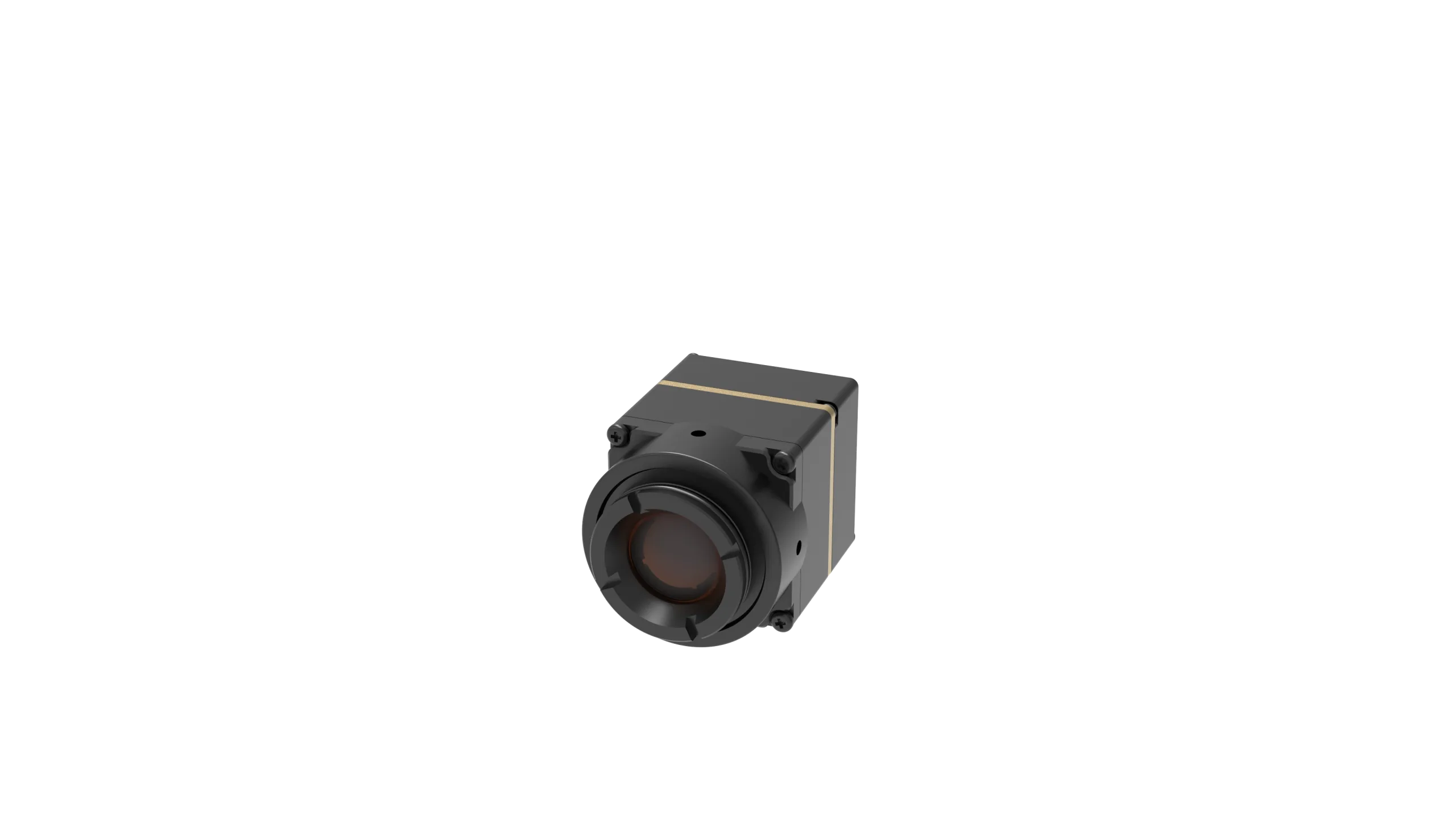
5. OEM Core Showcase: Camcuda MD-64CA 640×512 Thermal Camera Module
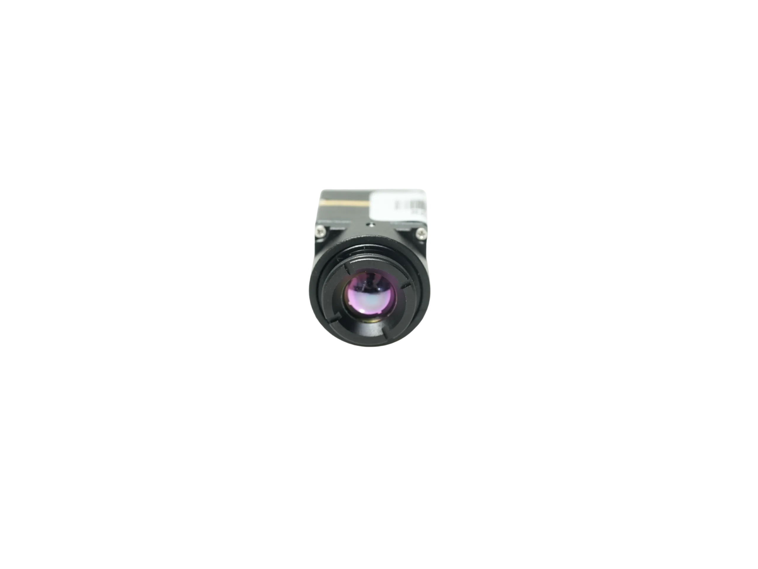
When you’re building thermal vision into small drone gimbals, uncrewed ground vehicles (UGVs), inspection tools, and tactical payloads, SWaP-C constraints dictate your hardware choices. The Camcuda MD-64CA is an uncooled VOx thermal imaging camera module built specifically for OEM integration, offering wide optical options, low latency, and straightforward electrical integration.
Camcuda MD-64CA 640 x 512 Uncooled VOx Thermal Imaging Camera Module
The MD-64CA matches a high-density 640 x 512 uncooled Vanadium Oxide (VOx) focal plane array with a 12 µm pixel pitch and high thermal sensitivity (≤30 mK NETD). Delivering a continuous 50 Hz video output in an ultra-lightweight 23.1 g bare-chassis form factor, it consumes under 0.7 W of power. Unlike legacy cores that require a strictly regulated 3.3V single rail, the MD-64CA features an integrated wide-voltage input stage (5–24V DC), saving you the space, heat, and cost of external DC-DC regulators across drone power systems and industrial equipment.
Factory-Fitted Lens Options & Optical Planning Reference
Optics are factory-collimated and mechanically secured to maintain boresight and focus through harsh vibration and shock environments. The operational matrix below details spatial performance across standard lens configurations based on Johnson Criteria modeling for a standard human target ($1.8 \times 0.5 \times 0.3\,\text{m}$):
| Focal Length | Field of View (H x V) | IFOV | Detection Range | Recognition Range | Identification Range |
|---|---|---|---|---|---|
| 4.1 mm | Extra-Wide Angle (Custom) | Confirmed in RFQ | Wide Area Survey | Close-Proximity | Obstacle Avoidance |
| 4.9 mm | 76.2° x 64.2° | 2.45 mrad | 476.0 m | 119.0 m | 60.0 m |
| 9.1 mm | 45.8° x 37.3° | 1.31 mrad | 884.7 m | 221.2 m | 110.6 m |
| 13.0 mm | 33.0° x 26.6° | 0.92 mrad | 1,263.9 m | 316.0 m | 158.0 m |
| 19.0 mm | 22.9° x 18.4° | 0.63 mrad | 1,847.2 m | 461.8 m | 230.9 m |
| 35.0 mm | 12.5° x 10.0° | 0.34 mrad | 3,402.8 m | 850.7 m | 425.4 m |
Interface & Electrical Specifications
- ✅ Flexible Video Output: Native support for CVBS Analog (Rx, Tx, CVBS, GND, VCC), USB UVC (USB-VDD, D-, D+, GND), or MIPI CSI-2 digital pipelines.
- ✅ Ultra-Low Core Latency: Sub-20 ms internal pipeline latency with automated shuttered Non-Uniformity Correction (NUC).
- ✅ Wide Input Power Subsystem: Nominal <0.7 W power draw across a wide 5–24V DC unregulated input range.
- ✅ Industrial Environmental Limits: Operating range from -20°C to +60°C in a compact 23.1 g bare-module envelope.
View Product Details & Pricing ➔
6. Portable Field Instrument: Camcuda Handheld Infrared Thermal Observation Device
For field teams, security personnel, infrastructure inspectors, and search-and-rescue units that need immediate situational awareness without building custom embedded carrier hardware, a fully packaged handheld thermal imager is the quickest path to deployment.
Camcuda Handheld Infrared Thermal Observation Instrument
The Camcuda Handheld Thermal Observation Instrument is an ergonomic, field-ready optical device built for perimeter security, tactical monitoring, predictive infrastructure auditing, and emergency response. Available in both 384 x 288 and 640 x 512 VOx configurations, it operates in the 8–14 µm spectral band with high thermal sensitivity (≤20 mK NETD @25°C, F1.0, 25 Hz).
Technical Specifications
| Sensor Core Type | VOx Uncooled Focal Plane Array (8–14 µm LWIR) |
|---|---|
| Resolution Options | 384 x 288 @ 12 µm / 640 x 512 @ 12 µm |
| Thermal Sensitivity (NETD) | ≤20 mK (@25°C, F#1.0, 25 Hz) |
| Frame Rate | 50 Hz continuous video output |
| Objective Lens Options | 25 mm / 35 mm / 50 mm F1.0 fast Germanium optics |
| Weight Class & Form Factor | Approx. 550 g ergonomic mobile enclosure |
| Target Applications | Outdoor perimeter monitoring, search & rescue, industrial auditing, safety surveys |
Field Configuration & RFQ Checklist
When putting together your RFQ or spec sheet, make sure your engineering and procurement teams confirm:
- 📌 Array Resolution: Select between the budget-friendly 384 x 288 array or the high-resolution 640 x 512 core for critical identification ranges.
- 📌 Germanium Objective Focal Length: Choose 25 mm for wide situational scans, 35 mm for balanced field work, or 50 mm for long-range observation.
- 📌 Power Ecosystem: Define your battery run-time requirements, hot-swap options, and field-charging hardware.
- 📌 Trade Compliance: Specify target destination requirements and compliance declarations before placing orders.
View Product Details & Pricing ➔
7. Architectural Specification Matrix: FLIR Boson vs. Camcuda Solutions
Picking the right thermal core means balancing thermal sensitivity, power consumption, input voltage flexibility, physical footprint, and supply chain lead times. The comparison table below lays out the industry-standard FLIR Boson alongside practical alternatives from the Camcuda ecosystem, including the MD-64CA OEM module, the Handheld Observation Device, and the 2-axis stabilized Camcuda 640 UAV Gimbal Camera.
| Architectural Parameter | FLIR Boson Baseline | Camcuda MD-64CA Module | Camcuda Handheld Instrument | Camcuda 640 UAV Gimbal |
|---|---|---|---|---|
| Detector Technology | Uncooled VOx Microbolometer | Uncooled VOx Focal Plane Array | Uncooled VOx Sensor | Stabilized VOx FPA Engine |
| Array Resolution | 640 x 512 / 320 x 256 | 640 x 512 | 384 x 288 or 640 x 512 | 640 x 512 |
| Pixel Pitch | 12 µm | 12 µm | 12 µm | 12 µm |
| Spectral Passband | 8 to 14 µm (LWIR) | 8 to 14 µm (LWIR) | 8 to 14 µm (LWIR) | 8 to 14 µm (LWIR) |
| Thermal Sensitivity (NETD) | ≤40 to 50 mK (std) / ≤20 mK (Pro) | ≤30 mK reference | ≤20 mK (@25°C, F1.0) | ≤30 mK reference |
| Max Frame Rate | 60 Hz (9 Hz export trims) | 50 Hz | 50 Hz | 50 Hz |
| Core Power Draw | ~0.5 W to 1.2 W (lens dependent) | <0.7 W reference | Integrated Battery Subsystem | Integrated Gimbal Supply |
| Input Voltage Range | 3.3 V DC (±5% strictly regulated) | 5 to 24 V DC Wide Input | Internal Recharging Circuit | Direct 3S–6S Drone Bus |
| Streaming Video Interfaces | CMOS Parallel, USB 3.0, MIPI | CVBS, USB UVC, or MIPI | Integrated Display / Micro-USB | Ethernet RTSP, Micro-HDMI, CVBS |
| Lens Focal Options | Factory Fixed: 4.9 to 73 mm | 4.1, 4.9, 9.1, 13, 19, 35 mm | 25, 35, 50 mm (F1.0) | Continuous Optical / Prime |
| Module Bare Weight | ~19 g to 34 g (lensless/lens) | 23.1 g | ~550 g (complete instrument) | ~280 g to 450 g (with 3-axis) |
8. SWaP-C Optimization, Optical Path Engineering & Johnson Criteria Sizing
In the shop, balancing SWaP-C across an airborne or mobile robotic system always comes down to trade-offs between physical aperture limits, thermal physics, and detection distance requirements.
Instantaneous Field of View (IFOV) & Angular Resolution: Spatial resolution in the LWIR spectrum is determined by your pixel pitch ($p$) and lens focal length ($f$). The Instantaneous Field of View (IFOV) formula is straightforward:
$$\text{IFOV (mrad)} = \frac{\text{Pixel Pitch } (p \text{ in } \mu\text{m})}{\text{Focal Length } (f \text{ in mm})}$$
A smaller IFOV gives you higher angular resolution at long distances, putting more pixels on target. But here’s the catch: as focal length goes up, the physical diameter, mass, and cantilever load of your Germanium optics grow rapidly. That extra weight requires bigger gimbal motors and higher drive currents, and it introduces stabilization lag under strong flight vibrations.
The Radiometric Aperture Penalty (F-Number Impact): In the 8–14 µm band, radiant flux reaching the microbolometer drops inversely with the square of the optical F-number:
$$\text{Irradiance on FPA } (E) \propto \frac{1}{4 \cdot (F\#)^2}$$
Moving from a fast F1.0 lens to an F1.2 or F1.4 lens cuts down incoming infrared photon energy. This raises your effective NETD and washes out low-contrast thermal details. Whenever you’re designing compact optics for low-contrast environments, prioritize high-transmission F1.0 antireflective-coated Germanium lenses to get the most out of your detector.
Thermal Dissipation & Structural Heatsinking: Uncooled VOx cores don’t need cryogenic Stirling coolers, but you still have to manage ambient internal thermal gradients. Rapid temperature swings across the camera housing create uneven heat patterns on the sensor array. This forces the camera into frequent Non-Uniformity Correction (NUC) shutter calibrations, freezing your video feed for hundreds of milliseconds right when you can’t afford it.
- ⚙️ Direct Chassis Coupling: Thermally couple the core’s metal housing directly to the main payload frame using high-conductivity thermal gap pads ($k \ge 3.0\,\text{W/m}\cdot\text{K}$).
- ⚙️ Component Isolation: Keep high-heat components—like power buck-boost regulators, battery packs, and edge AI compute chips—away from the microbolometer housing.
- ⚙️ Stress-Free Mechanical Mounting: Use balanced mechanical mounting points so thermal expansion doesn’t transfer physical strain into the sensor’s ceramic package.
9. Deep-Dive Technical FAQ & Hardware Troubleshooting
What are the primary hardware challenges when interfacing thermal cores like FLIR Boson with Jetson or Raspberry Pi?
How do developers configure multi-camera hardware synchronization (EXT_SYNC) for thermal stereo vision?
What are the critical SWaP trade-offs when evaluating LWIR OEM camera cores for drone payloads and robotics?
How does optical F-number affect LWIR sensor performance and NETD sensitivity?
📚 References & Further Reading
- 🔗 Industry Standard: A3 Camera Link Standard Specification
- 🔗 AI Acceleration: Hailo AI Embedded Neural Processors
- 🔗 Related Guide: Camcuda 640×512 UAV Gimbal Camera Integration
- 🔗 Thermal Cores Catalog: Explore Uncooled OEM Thermal Imaging Cores
- 🔗 Company Portal: Camcuda Advanced Infrared Systems